Extracting Demographic and Diagnostic Sample Attributes from NCI’s Genomic Data Commons
Michael Kesling 7/25/2019
Introduction
In order to correctly select the pertinent RNA-Seq samples from The Cancer Genome Atlas (TCGA) project, it’s necessary to access attribute data about the samples from the NCI’s Genomic Data Commons (GDC), where the data are now warehoused (https://gdc.cancer.gov).
A Bioconductor package named ‘GenomicDataCommons’ is utilized here in order to explore and then extract the relevant fields of sample attributes. The ‘BiocManager’ package must first be installed in order to install bioconductor packages.
Note:
Some of the code is not shown on the GitHub website. One needs to look at the R Markdown file to view all of the code.
Understanding TCGA Identifiers
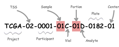
Each RNA-Seq file that was generated by TCGA, whether it was obtained directly through GDC, from the Wang publication of cross-study normalized data, or other studies, is identified through its TCGA identifier. This identifier gives important information regarding the type of sample used, and is essential for mapping attribute data on GDC to other published studies.
We’ll look at the structure of the TCGA identifier to determine what information we need to uniquely identify a human patient.
| Label | Identifier_for | Value | Value_Description | Possible_Values |
|---|---|---|---|---|
| TSS | Tissue Source Site | 2 | GBM (brain tumor) sample from MD Anderson | see https://gdc.cancer.gov/resources-tcga-users/tcga-code-tables/tissue-source-site-codes for complete list |
| Participant | Study Participant (Patient) | 14 | The 14th participant from the GBM Study of MD Anderson | Any alph-numeric value |
| Sample | Sample Type | 1 | A solid tumor | Tumor types range from 01-09, normal types from 10-19, and control samples from 20-29. See https://gdc.cancer.gov/resources-tcga-users/tcga-code-tables/sample-type-codes |
While other fields in the TCGA identifier may be important, the “TSS”, “Participant”, and “Sample” fields are sufficient for identifying the desired sample attributes of individual patients on GDC.
Exploring GDC Sample Attributes
We using the Vignette for the GenomicDataCommons package to explore and query the GDC data.
As the sample attributes of Demographics (characteristics of the human patient such as age, sex, race, etc.) and Diagnoses (characteristics of the tumor/healthy sample such as stage of cancer, new diagnosis/recurrence, etc.) all fall under the umbrella of the cases, we’ll access our data through the GenomicDataCommons function cases().
Let’s start out by simply asking how many different cases are stored by GDC:
GenomicDataCommons::cases() %>% GenomicDataCommons::count()
## [1] 34893
We see that there are over 34,000 cases as of July 2019.
Identifying Breast Cancer Project ID
As we’re focusing on breast cancer, and the samples are grouped into projects according to the type of cancer, we’ll need to determine the correct identifier for subsetting all cases by those involving breast cancer.
First, we need to determine the exact field and identifier for the Project ID. We’ll use the grep() function to try and find that field.
project_fields <- grep('proj', available_fields('cases'), value=TRUE)
print(project_fields)
##  [1] "project.dbgap_accession_number"
##  [2] "project.disease_type"
##  [3] "project.intended_release_date"
##  [4] "project.name"
##  [5] "project.primary_site"
##  [6] "project.program.dbgap_accession_number"
##  [7] "project.program.name"
##  [8] "project.program.program_id"
##  [9] "project.project_id"
## [10] "project.releasable"
## [11] "project.released"
## [12] "project.state"
## [13] "tissue_source_site.project"
It appears that the exact field name is project.project_id. Let’s determine what value a project ID would have for a breast cancer sample.
projClasses <- cases() %>%
   facet('project.project_id') %>%
   aggregations()
head(projClasses$project.project_id)
##             key doc_count
## 1         FM-AD     18004
## 2    TARGET-NBL      1120
## 3     TCGA-BRCA      1098
## 4 MMRF-COMMPASS       995
## 5    TARGET-AML       988
## 6     TARGET-WT       652
We can see that one of the most popular entries under ‘project_id’ is ‘TCGA-BRCA’, giving 1098 cases of breast cancer as of July 2019. We will focus on this dataset going forward.
Identifying TCGA identifier and Downloading Sample Data
We need to ensure that for the breast cancer sample attributes we download, that there is a TCGA ID related to the case number. We’ll need that for identifying the right RNA-Seq identifiers in other publications later on.
The ‘case_id’ is needed for joining data across tables or object, but its format is not in the TCGA format. e.g. 87b85935-a058-44ad-8fb6-8511130eaffe
We start by figuring out what the ‘sample_id’ might be called in GDC. We’ll use grep() for this:
sample_fields <- grep('sample_id', available_fields('cases'), value=TRUE)
print(sample_fields)
## [1] "sample_ids" "samples.sample_id" "submitter_sample_ids"
More than one identifier will serve our purpose, as long as it begins with TCGA, and contains the TSS, Participant, and Sample fields. Based on iterating through this code previously, it was found that submitter_sample_ids will suffice for our purpose, as shown with the following code. We are going to pull all the sample attribute data that we’ll need, and we’ll look at it step-by-step below, starting with the submitter_sample_ids.
expands = c("diagnoses","annotations",
            "demographic","exposures")
brcaResults <- cases() %>%
   GenomicDataCommons::filter(~ project.project_id == 'TCGA-BRCA') %>%
   GenomicDataCommons::select("submitter_sample_ids") %>%
   GenomicDataCommons::expand(expands)   %>%
   response_all()

print(c("`f06f09f3-8133-4a92-ac86-fbe64295e0d8` ->", (list(brcaResults$results$submitter_sample_ids$`f06f09f3-8133-4a92-ac86-fbe64295e0d8`))))
## [[1]]
## [1] "`f06f09f3-8133-4a92-ac86-fbe64295e0d8` ->"
##
## [[2]]
## [1] "TCGA-E9-A1ND-10A" "TCGA-E9-A1ND-01Z" "TCGA-E9-A1ND-01A"
## [4] "TCGA-E9-A1ND-11A"
We see that the TSS, Participant, and Sample fields are present in these submitter_sample_ids. • The case_id begins with ‘f06f…’ • We see that it maps to 4 distinct submitter_sample_ids. Each one begins with ‘TCGA-E9-A1ND’. • “E9” is the code for the “Breast Invasive Carcinoma” study at the Asterand Biosciences. • “A1ND” is the patient/participant code for that study. We notice that these values are the same for all 4 submitter_sample_id codes, which says that all 4 samples were generated from the same patient. • 2 of the sample_code fields are “01Z” and “01A”. “01”” refers to a “Primary Solid Tumor”, and A and Z refer to the fact that these are 2 separate samples. I assume that are labeled A and Z (rather than A and B) because they are the 1st and 2nd Primary Solid Tumors out of a total of 2 (rather than the 1st and 2nd out of several). • We also notice that this patient has 2 other samples whose sample type is 10 = “Blood-Derived Normal Cell” and 11 = “Solid Tissue Normal”. That means that 2 non-cancerous controls were taken from this patient, in addition to the 2 primary solid tumor samples taken.
Exploring brcaResults Data Object
brcaResults is the name of the GDCcasesResponse object, which is fundamentally a list, that was returned from the data query to GDC. We’d like to understand how the demographic, diagnoses, exposure, and annotations objects are organized.
dem <- class(brcaResults$results$demographic)
diag <- class(brcaResults$results$diagnoses)
annot <- class(brcaResults$results$annotations)
exp <- class(brcaResults$results$exposures)
print(c("demographic ->", dem, "diagnostic ->", diag, "exposures -> ", exp, "annotations -> ", annot))
## [1] "demographic ->"  "data.frame"      "diagnostic ->"   "list"
## [5] "exposures -> "   "list"            "annotations -> " "list"
We can see that demographic is a data frame. (It contains the demographic data directly.) Right now, we’ll explore how the annotations and diagnoses lists are laid out, and how sparse they are.
lists <- c("brcaResults$results$annotations", "brcaResults$results$diagnoses")
for(listName in lists){
   numAnnotNull <- 0
   resNum <- 0
   for(result in eval(parse(text=listName))){
      resNum = resNum+ 1
      if(is.null(result)){
         numAnnotNull = numAnnotNull + 1
      }
   }
   print(paste("The fraction of ", listName, " records that are empty is ", numAnnotNull/resNum))
}
## [1] "The fraction of  brcaResults$results$annotations  records that are empty is  0.973588342440802"
## [1] "The fraction of  brcaResults$results$diagnoses  records that are empty is  0.000910746812386157"
Clearly, the annotations list is almost completely empty, so we’ll want to ignore it for this work, while the diagnoses list is almost entirely populated and we’ll want to use it.
The structure of the exposures list of dataframes is a bit different, as empty fields are still populated with a header. Let’s see how well it’s populated:
fields <- c("cigarettes_per_day", "alcohol_intensity", "bmi", "years_smoked")

numAnnotNull <- 0
resNum <- 0
for(result in brcaResults$results$exposures){
   if(!is.null(result)){
      resNum = resNum + 1
      if(all(is.na(result[fields])) & result$alcohol_history=="Not Reported"){
         numAnnotNull = numAnnotNull + 1
      }
   }
}
print(paste("The fraction of the exposures records that are empty is ", numAnnotNull/resNum))
## [1] "The fraction of the exposures records that are empty is 1"
So clearly the exposures list has no useful information.
Selecting Relevant Fields in demographic and diagnoses data objects
Now that we’ve decided to not use the annotations and exposures data lists, we’ll see what fields in the demographic and diagnoses objects we might be interested in.
Let’s see what fields are available in the demographic data frame:
colnames(brcaResults$results$demographic)
##  [1] "updated_datetime" "created_datetime" "gender"
##  [4] "state"            "submitter_id"     "year_of_birth"
##  [7] "race"             "days_to_birth"    "ethnicity"
## [10] "vital_status"     "demographic_id"   "age_at_index"
## [13] "year_of_death"    "days_to_death"
As we’re interested in characteristics about the patients and not the time when the data were entered into the GDC database, we’ll subset these fields and look at the first few rows in tibble format.
importantDemographicFields <- c("gender", "race", "days_to_birth", "ethnicity",
                                "vital_status", "age_at_index", "days_to_death",
                                "year_of_birth", "year_of_death")
brcaData1098 <- brcaResults$results$demographic[importantDemographicFields]
brcaData1098 <- cbind(rownames(brcaData1098), brcaData1098)
colnames(brcaData1098) <- c("sampleId", importantDemographicFields)
brcaData1098 <- as_tibble(brcaData1098)
head(brcaData1098, n=4)
## # A tibble: 4 x 10
##   sampleId                             gender race
##   <fct>                                <chr>  <chr>
## 1 87b85935-a058-44ad-8fb6-8511130eaffe female white
## 2 dd96a9c7-899c-47cd-a0f9-b149ed07a5d6 female white
## 3 3f834fa7-6d7b-4b85-98c0-5c55d55b6c95 female black or african american
## 4 451e1a67-47e6-4738-99d7-fb7771ef61a3 female white
##   days_to_birth ethnicity              vital_status age_at_index
##           <int> <chr>                  <chr>               <int>
## 1        -30830 not hispanic or latino Alive                  84
## 2        -19822 not hispanic or latino Alive                  54
## 3        -13982 not hispanic or latino Dead                   38
## 4        -26941 not hispanic or latino Dead                   73
##   days_to_death year_of_birth year_of_death
##           <int>         <int>         <int>
## 1            NA          1926            NA
## 2            NA          1956            NA
## 3          1993          1957          2000
## 4          3126          1921          2002
We can see that these selected fields are all important, and we can also deduce that “age_at_index” refers to the age at which the patient was diagnosed with breast cancer. The 4th patient in the output above was born in 1921, was 73 years old at “age_at_index”, had 3126 days_to_death (3126/365=8.5 years), and died in 2002. 1921 + 73 + 8.5 = 2002.5.
Now let’s look at what fields in the diagnoses list of dataframes might be of interest.
colnames(brcaResults$results$diagnoses$`87b85935-a058-44ad-8fb6-8511130eaffe`)
##  [1] "year_of_diagnosis"
##  [2] "classification_of_tumor"
##  [3] "last_known_disease_status"
##  [4] "updated_datetime"
##  [5] "primary_diagnosis"
##  [6] "submitter_id"
##  [7] "tumor_stage"
##  [8] "age_at_diagnosis"
##  [9] "morphology"
## [10] "days_to_last_known_disease_status"
## [11] "created_datetime"
## [12] "prior_treatment"
## [13] "state"
## [14] "days_to_recurrence"
## [15] "diagnosis_id"
## [16] "tumor_grade"
## [17] "icd_10_code"
## [18] "days_to_diagnosis"
## [19] "tissue_or_organ_of_origin"
## [20] "progression_or_recurrence"
## [21] "prior_malignancy"
## [22] "synchronous_malignancy"
## [23] "site_of_resection_or_biopsy"
## [24] "days_to_last_follow_up"
Of these diagnoses fields, we’ll use the following: “primary_diagnosis”, “tumor_stage”, “age_at_diagnosis”, “morphology”, “prior_treatment”, “tissue_or_organ_of_origin”, “prior_malignancy”.
‘tumor_grade’ is not reported, ‘icd_10_code’ is always C50.9 (invasive breast cancer), and “days_to_recurrence” is always NA, so they won’t be used.
importantDiagnosisFields <- c("primary_diagnosis", "tumor_stage", "age_at_diagnosis",
                              "morphology", "prior_treatment",  "tissue_or_organ_of_origin",
                              "prior_malignancy")

brcaSampleIDs1098 <- names(brcaResults$results$diagnoses)

diagnostics <- brcaResults$results$diagnoses[[brcaSampleIDs1098[1]]][importantDiagnosisFields]
sampleId <- c(brcaSampleIDs1098[[1]])
for(id in brcaSampleIDs1098[2:length(brcaSampleIDs1098)]){
   record <- brcaResults$results$diagnoses[[id]][importantDiagnosisFields]
   if(!is.null(record)){                                   # handles NULL record
      diagnostics <- rbind(diagnostics, record)
      sampleId <- c(sampleId, id)
   }
}
diagnostics <- cbind(sampleId, diagnostics)
diagnostics <- as_tibble(diagnostics)
Joining together the 2 Tibbles
We’ll now want to join together all the columns from the brcaData1098 tibble, which contains the demographic attributes of interest, and the diagnostics tibble, which contains the cancer tumor (or healthy sample) attributes of interest.
suppressWarnings(brcaSampleData1097 <- inner_join(brcaData1098, diagnostics))
## Joining, by = "sampleId"
As there was a record that existed in demographics that did not exist in diagnoses, that row was removed, bringing the number of patients in our full breast cancer dataset to 1097. The Tibble storing the data is called brcaSampleData1097.
Adding TCGA Identifiers to Dataframe
One other piece of information we’ll need is to add on the list of TCGA IDs associated with each sampleId.
# set up first row of expanded data frame/tibble:
smpId <- as.character(brcaSampleData1097[1,"sampleId"])
tcgaId <- brcaResults$results$submitter_sample_ids[smpId]
tmp <- cbind(brcaSampleData1097[1,], paste(unlist(tcgaId), collapse=";")) #tmp dataframe

# loop through other rows and add them
for(i in 2:dim(brcaSampleData1097)[1]){
   smpId <- as.character(brcaSampleData1097[i,"sampleId"])
   tcgaId <- brcaResults$results$submitter_sample_ids[smpId]
   tmp <- rbind(tmp, cbind(brcaSampleData1097[i,], paste(unlist(tcgaId), collapse=";")))
}

# add new column name, convert to tibble and print first 4 rows:
names(tmp)[names(tmp) == 'paste(unlist(tcgaId), collapse = ";")'] <- 'tcgaID'
brcaSampleData1097 <- as_tibble(tmp)
head(brcaSampleData1097, n=4)
## # A tibble: 4 x 18
##   sampleId                             gender race
##   <chr>                                <chr>  <chr>
## 1 87b85935-a058-44ad-8fb6-8511130eaffe female white
## 2 dd96a9c7-899c-47cd-a0f9-b149ed07a5d6 female white
## 3 3f834fa7-6d7b-4b85-98c0-5c55d55b6c95 female black or african american
## 4 451e1a67-47e6-4738-99d7-fb7771ef61a3 female white
##   days_to_birth ethnicity              vital_status age_at_index
##           <int> <chr>                  <chr>               <int>
## 1        -30830 not hispanic or latino Alive                  84
## 2        -19822 not hispanic or latino Alive                  54
## 3        -13982 not hispanic or latino Dead                   38
## 4        -26941 not hispanic or latino Dead                   73
##   days_to_death year_of_birth year_of_death
##           <int>         <int>         <int>
## 1            NA          1926            NA
## 2            NA          1956            NA
## 3          1993          1957          2000
## 4          3126          1921          2002
##   primary_diagnosis                       tumor_stage  age_at_diagnosis
##   <chr>                                   <chr>                   <int>
## 1 Mucinous adenocarcinoma                 stage iia               30830
## 2 Infiltrating duct carcinoma, NOS        stage iib               19822
## 3 Lobular carcinoma, NOS                  stage iiia              13982
## 4 Infiltrating duct and lobular carcinoma not reported            26941
##   morphology prior_treatment tissue_or_organ_of_origin prior_malignancy
##   <chr>      <chr>           <chr>                     <chr>
## 1 8480/3     No              Breast, NOS               no
## 2 8500/3     No              Breast, NOS               no
## 3 8520/3     No              Breast, NOS               no
## 4 8522/3     No              Breast, NOS               no
##   tcgaID
##   <fct>
## 1 TCGA-D8-A1XV-10A;TCGA-D8-A1XV-01A;TCGA-D8-A1XV-01Z
## 2 TCGA-D8-A1JB-10A;TCGA-D8-A1JB-01Z;TCGA-D8-A1JB-01A
## 3 TCGA-B6-A0IE-01A;TCGA-B6-A0IE-01Z;TCGA-B6-A0IE-10A
## 4 TCGA-B6-A0RP-01A;TCGA-B6-A0RP-01Z;TCGA-B6-A0RP-10A
Exporting Full Set of Breast Cancer Sample Attributes
As part of our work, we’ll want to work on the full set of breast cancer samples. So we’ll export the brcaSampleData1097 data frame at this point for later use.
write.table(brcaSampleData1097, "TCGA_Attributes_full.txt", sep="\t", row.names = FALSE)
Exploring Sub-Classes of Breast cancer
For some work we’ll do on data simulation, we’ll subset the full attribute data frame to those having specific attributes.
We select out only those cases that are breast cancer and see what data are available to us:
cases() %>%
   GenomicDataCommons::filter( ~ project.project_id == 'TCGA-BRCA') %>%   # '~' needed
   facet('disease_type') %>%
   aggregations() %>%
   head()
## $disease_type
##                                     key doc_count
## 1          Ductal and Lobular Neoplasms      1054
## 2 Cystic, Mucinous and Serous Neoplasms        16
## 3          Complex Epithelial Neoplasms        14
## 4             Epithelial Neoplasms, NOS         5
## 5          Adenomas and Adenocarcinomas         3
## 6             Fibroepithelial Neoplasms         2
## 7               Squamous Cell Neoplasms         2
## 8  Adnexal and Skin Appendage Neoplasms         1
## 9                  Basal Cell Neoplasms         1
We see that ‘Ductal and Lobular Neoplasms’ cover almost all cases. Analysis of the most common values in the field primary_diagnosis shows that 778 samples have the specific diagnosis “Infiltrating duct carcinoma, NOS” (see below).
tbl <- table(brcaSampleData1097$primary_diagnosis)
kable(head(sort(tbl, decreasing=TRUE), n=5))
| Var1 | Freq |
|---|---|
| Infiltrating duct carcinoma, NOS | 778 |
| Lobular carcinoma, NOS | 201 |
| Infiltrating duct and lobular carcinoma | 28 |
| Infiltrating duct mixed with other types of carcinoma | 19 |
| Mucinous adenocarcinoma | 16 |
Subsetting Samples
In an analysis being performed modeling healthy and tumor samples, limitations are being placed on which samples will be used to reduced confounding.
From the full brcaSampleData1097 breast cancer dataset, we’ll filter out: (a) those samples that are not ‘Infiltrating duct carcinoma, NOS’ (b) men (12 samples in total) (c) those from women not between ages 40-49 at the time of diagnosis (d) those that have previous treatments or previous diagnoses (e) those from women who are not white and those who are Latino
brcaDuctF40W_86 <- brcaSampleData1097 %>%                       # start with 1097 samples
   dplyr::filter(primary_diagnosis=='Infiltrating duct carcinoma, NOS') %>% # 778 remaining
   dplyr::filter(gender=="female") %>%                                      # 767 remaining
   dplyr::filter(age_at_index >= 40 & age_at_index < 50) %>%                # 159 remaining
   dplyr::filter(race=="white") %>%                                         # 100 remaining
   dplyr::filter(ethnicity=="not hispanic or latino")                       #  86 remaining
Writing Desired Attributes to a File
We will write the brcaDuctF40W_86 dataframe to a corresponding file.
write.table(brcaDuctF40W_86, "brcaDuctF40W_86.txt", sep="\t", row.names=FALSE)
This file can now be used to study samples from various studies.